Supply chain contracts

Péter Egri

    |    

Outline

Contracts

Wholesale contract

Buyback contract

Revenue sharing contract

Call option contract

Contracts with dominant supplier

Profit sharing

    |    

The model

Parameters

Retail price (R): the unit price of the products on the market.

Wholesale price (W): the unit price of the products paid for the supplier.

Production cost (C): the unit production cost of the supplier.

Salvage value (V): the unit salvage value for the remaining products at the retailer.

Goodwill penalty cost (G): the unit cost for shortage.

Variables

Demand (D): stochastic variable.

Order quantity (Q): decision variable of the retailer.

Assumptions

Two players: the retailer (decision maker) and the supplier

Complete information

Risk neutral (expected profit maximizer) players

One period (newsvendor model)

The retailer applies Make-To-Forecast

The supplier applies Make-To-Order (with forced compliance)

V≤C≤R

    |    

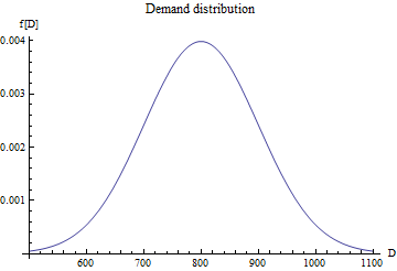
Demand

The demand is stochastic with probability distribution function f[x], cumulative distribution function F[x], expected value μ and standard deviation σ. We assume that F[x] is strictly increasing.
In the illustrations, we will use the following normal distribution:

Out[42]=

    |    

Notations

Let us introduce the following functions:
Expected sales:

Expected remaining inventory:

Expected lost sales:

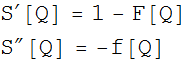
We will also require the first and second derivatives of S[Q]:

    |    

Supply chain optimum

If we denote the expected payment trasfer between the retailer and the supplier with T, then the expected profit of the supplier becomes

the expected profit of the retailer is

and the the total supply chain profit is

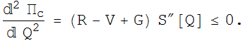
Note that is independent from the payment between the retailer and the supplier.
is concave function of Q, since

The unique optimal production quantity () of the supply chain is therefore given by the equation

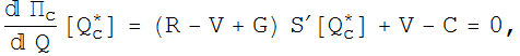
i.e.,

    |    

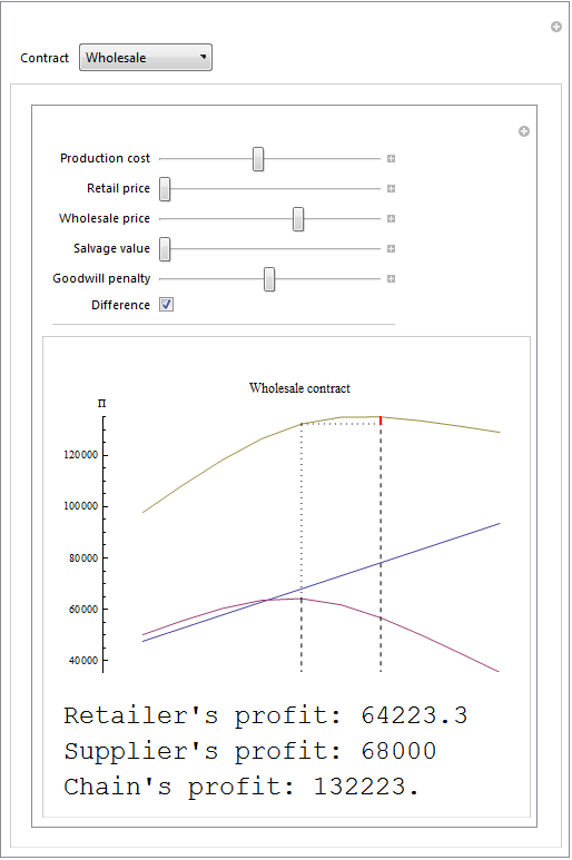
Wholesale contract

With a wholesale contract the retailer pays after the quantities ordered:

We assume that C≤W≤R. The profit of the retailer is therefore

Notice the similarity between this function and (1): the only difference is that the purchase cost (W) is used instead of the production cost (C). Therefore the retailer's optimal order quantity becomes

Note that ≤, and = only if W=C, in which case the profit of the supplier is zero.
The problem of the wholesale contract is that the retailer takes all risks, and this results in an order quantity lower than the supply chain optimal.

    |    

Wholesale contract illustration

.

In[45]:=

Out[45]=

    |    

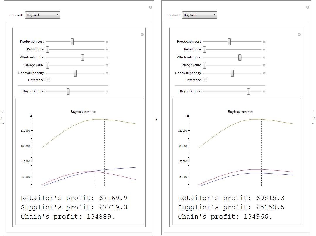
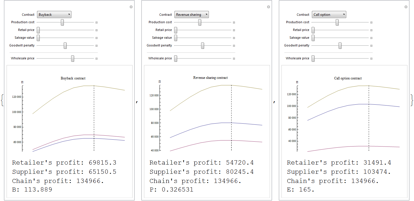
Buyback contract

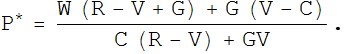
In order to inspire the retailer ordering more, the supplier offers to buy back the remaining obsolete inventory with the unit buyback price B (V≤B≤W). For the retailer, this seems a higher "salvage value", therefore it is equivalent with the following expected payment:

We assume that C≤W≤R. The profit of the retailer is therefore

The retailer's optimal order quantity becomes

The channel is coordinated ( =) if and only if

    |    

Buyback contract illustration

.

In[46]:=

Out[46]=

    |    

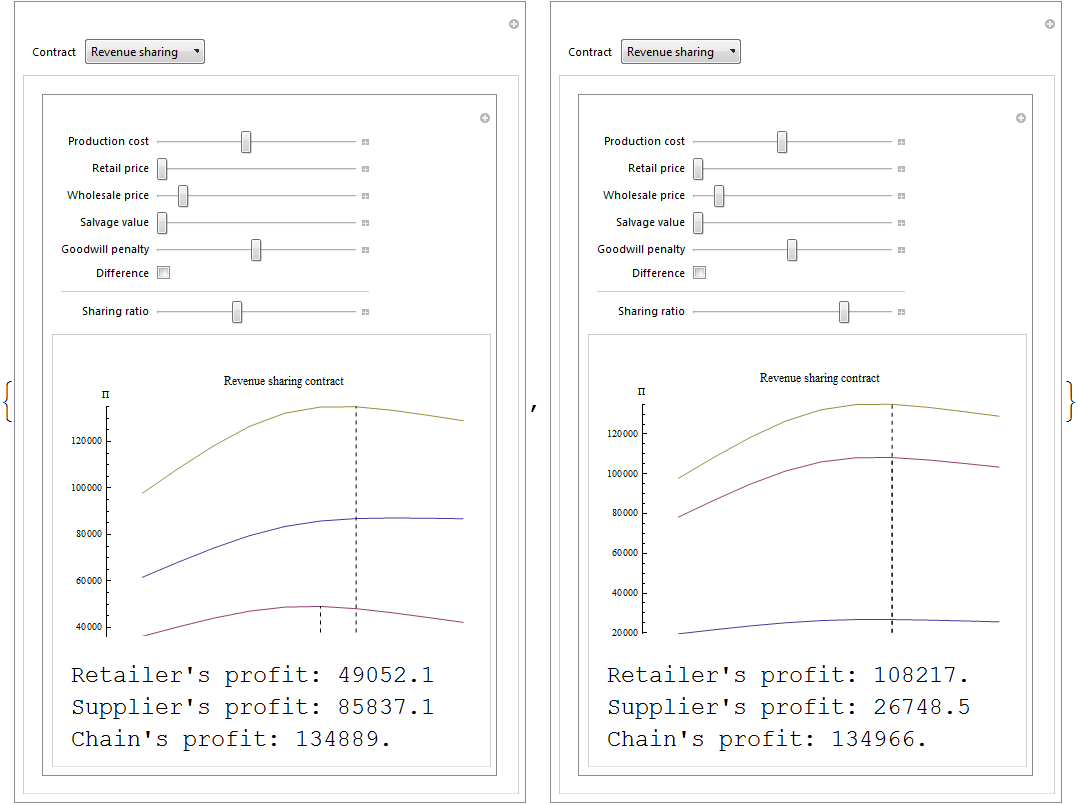
Revenue sharing contract

In order to inspire the retailer ordering more, the supplier offers lower wholesale price, but takes (1-P) percentage of the retailer's revenue. This results the following expected payment:

The profit of the retailer is

The retailer's optimal order quantity becomes

The channel is coordinated ( =) if and only if

    |    

Revenue sharing contract illustration

.

In[47]:=

Out[47]=

    |    

Call option contract

With this contract, the retailer buys Q call options with unit price W, and when the demand materializes, it can buy at most Q products with E unit execution price.

The profit of the retailer is

The retailer's optimal order quantity becomes

The channel is coordinated ( =) if and only if

    |    

Call option contract illustration

.

In[48]:=

Out[48]=

    |    

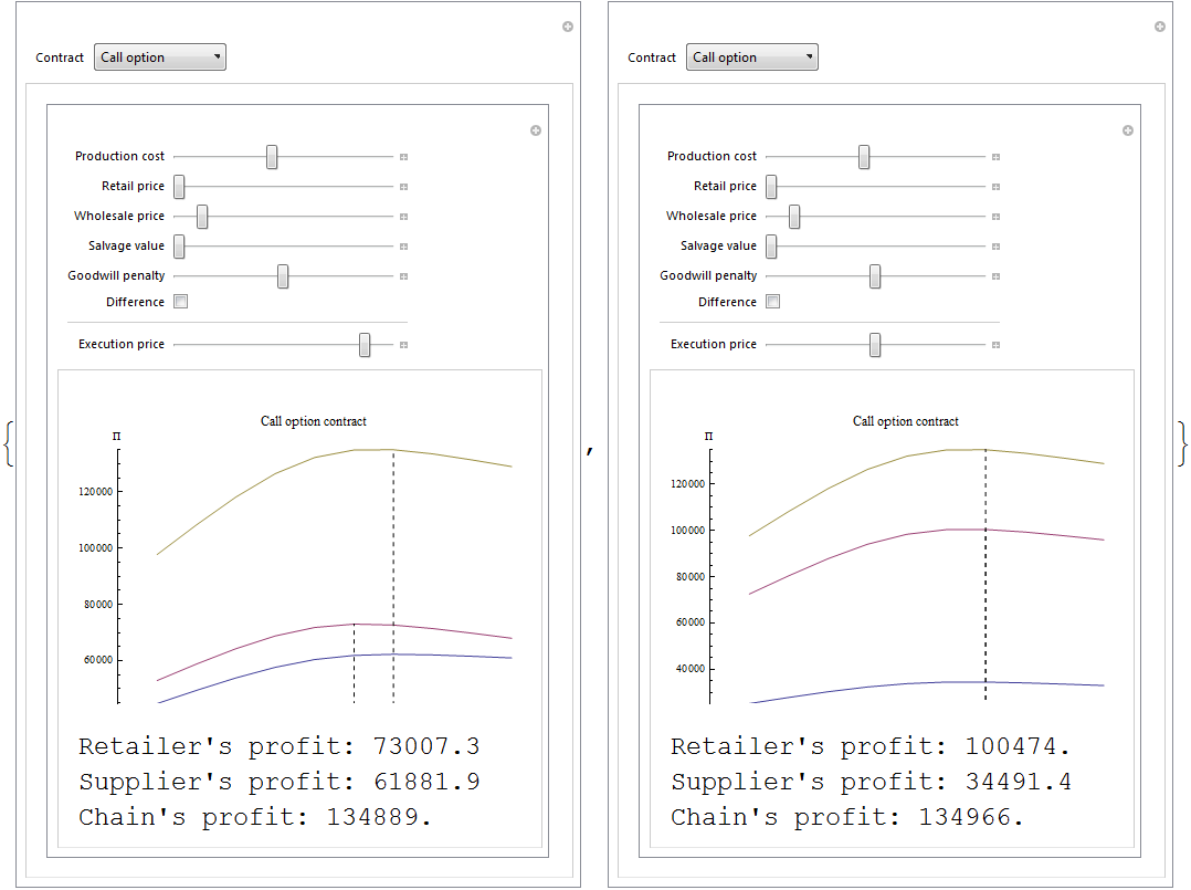
Other contracts

There are several other common contract, but they are slightly more difficult to analyze. Some examples are

Quantity flexibility contract: the retailer buys Q products with W unit price, but if D<Q, the supplier buys back at most K Q products at unit price W, where 0≤K≤1.

Sales rebate contract: the retailer pays W unit price if Q is smaller than a predefined limit L, and pays a smaller unit price for all products above the limit.

Quantity discount contract: instead of a W price, the retailer pays according to a decreasing function W[Q].

    |    

Contracts with dominant supplier

In this part we study the supply chain with a dominant supplier, i.e., the supplier determines the contract parameters. (The other possibility when the retailer is dominant is simpler, since we assume forced compliance, thus the retailer is interested in lowering the prices to the possible limit.) Here we deal only with the wholesale contract, since it has only one parameter, which makes the problem relatively easy.
We have seen that if the suppliers sets the wholesale price W, the the retailer's optimal order quantity will be

This defines a bijection between W and Q, and thus for comfortability, we can consider that the supplier decides Q and then W is given by

The supplier's profit is then becomes

The supplier intends to maximize this function, which task is analitically harder than maximising the retailer's or the channel's profit. We can only show a sufficient condition for a unique optimum by regarding the derivative of :

If this derivative is strictly decreasing, then the profit function has a unique maximum on [0,∞]: from (2) it can be seen that , and (when V<C).
Since 1 - F[Q] is strictly decreasing, we need that would be increasing. This property is called Increasing Generalized Failure Rate (IGFR), and several distributions have this property, including the normal distribution.
Note that for determining the optimal wholesale price, the supplier must know the distribution of the demand. As we have seen previously, the supply chain's optimal parameters are independent from the distribution, for all four contracts.

    |    

Wholesale contract with dominant supplier illustration

.

In[49]:=

Out[49]=

    |    

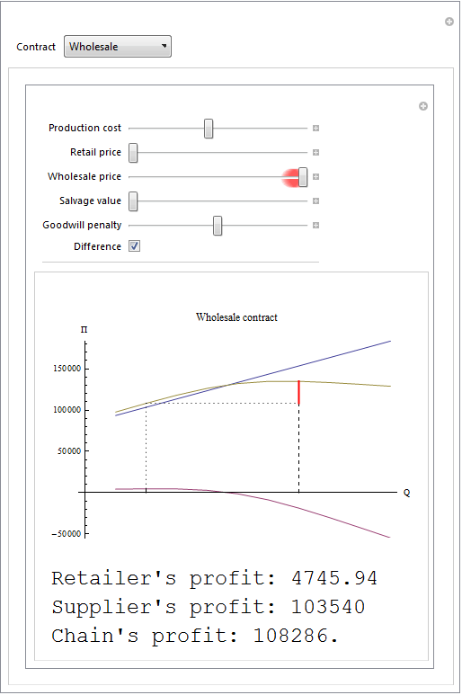
Profit sharing

Let us now consider the contract with the channel coordinating parameters. We have seen that with the wholesale price contract, the channel coordinating parameter results in zero profit for the supplier. With the buyback, revenue sharing and option contracts, the channel coordinating , and parameters depend on the wholesale price. Therefore W can be considered as the parameter that controls the allocation of the optimal supply chain profit between the partners.

In[50]:=

Out[50]=

    |    

Created with Wolfram Mathematica 7.0